Operationalising Deep Learning (CNN) Model using ONNX, Keras & Flask: A Starter Guide
 By Dr. Mufajjul Ali, Data Solution Architect at CSU UK
ONNX (Open Neural Network Exchange) is an open format that represents deep learning models. It is a community project championed by Facebook and Microsoft. Currently there are many libraries and frameworks which do not interoperate; hence, the developers are often locked into using one framework or ecosystem. The goal of ONNX is to enable these libraries and frameworks to work together by sharing of models.
Why ONNX?
ONNX provides an intermediate representation (IR) of models (see below), whether a model is created using CNTK, TensorFlow or another framework. The IR representation allows deployment of ONNX models to various targets, such as IoT, Windows, Azure or iOS/Android.
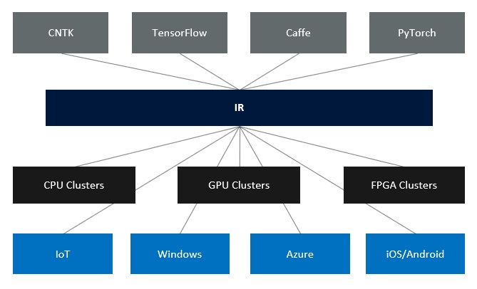
The intermediate representation provides data scientist with the ability to choose the best framework and tool for the job at hand, without having to worry about how it will be deployed and optimized for the deployment target.
How should we use ONNX?
ONNX provides two core components:
- Extensible computational graph model. This model is represented as an acyclic graph, consisting of a list of nodes with edges. It also contains metadata information, such as author, version, etc.
- Operators. These form the nodes in a graph. They are portable across the frameworks and are currently of three types.
- Core Operators - These are supported by all ONNX-compatible products.
- Experimental Operators - Either supported or deprecated within few months.
- Custom Ops - which are specific to a framework or runtime.
Where should we use ONNX?
ONNX emphasises reusability, and there are four ways of obtaining ONNX models:
- Public Repository
- Custom Vision Services
- Convert to ONNX model
- Create your own in DSVM or Azure Machine Learning Services
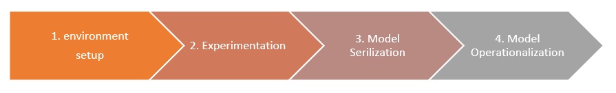
For custom models and converters, please review the currently supported export and import model framework. We'll go through a step-by-step guide for creating a custom model, convert it into ONNX then operationalise it using Flask.
Step-by-step Guide to Operationalizing ONNX models
The focus areas are as follows:
- How to install ONNX on your Machine
- Creating a Deep Neural Network Model Using Keras
- Exporting the trained model using ONNX
- Deploying ONNX in Python Flask using ONNX runtime as a web service
We are using the MNIST dataset for building a deep ML classification model.
Step 1: Environment setup
Conda is an open-source package management system and management environment, primarily designed for Python, that quickly installs, runs and updates packages and their dependencies.
It is recommended that you use a separate Conda environment for the ONNX installation, as this would avoid potential conflicts with existing libraries. Note: If you do not have Conda installed, you can install it from the official website.
Create & Activate Conda Environment
To create a new Conda environment, type the following commands in the terminal window:
 1 conda create -n onnxenv python=3.6.6
2 Source activate onnxenv (Mac/Linux)
3 activate onnxenv (Windows)
Line 1 creates an environment called ‘onnxenv’ for Python version 3.6.6 and installs all the libraries and their dependencies. It is possible to install other versions simply by referencing the version number. Lines 2-3 activate the environment depending on the choice of platform.
Installing ONNX/Keras and other Libraries
The core python library for ONNX is called onnx and the current version is 1.3.0.
 1 pip install onnx
2 pip install onnxmltools
3 pip install onnxruntime
4 pip install Keras
5 pip install matplotlib
6 pip install opencv_python
Lines 1-3 install the libraries that are required to produce ONNX models and the runtime environment for running an ONNX model. The ONNX tools enable converting of ML models from another framework to ONNX format. Line 4 installs the Keras library which is a deep machine learning library that is capable of using various backends such CNTK, TensorFlow and Theano.
Step 2: Preparing the Dataset
In this example, you will be creating a Deep Neural Network for the popular MNIST dataset. The MNIST dataset is designed to learn and classify handwritten characters.
There is some prep work required on the dataset before we can start building and training the ML model. We need to load the MNIST dataset and split them between train and test sets. Line 1 below loads the dataset and provides a default split of 60:40 (60% training, and 40% testing).
 …
1 (train_features, train_label), (test_features, test_label) = mnist.load_data()…
2 train_features = train_features.astype('float32')
3 train_features/=255 …
6 if backend.image_data_format() == 'channels_first':
7 #set channel at the begining
8 else:
9 #set the channel at the end
The total split of the data is [60000, 28, 28] [60000,] training dataset, and [10000, 28, 28] [10000,] testing dataset. Lines 2-5 ensure that datatype is float and ranges between 0.0-1.0.
Since we are dealing with grayscaled images, there is only one channel. Lines 6-7 check to see if the channel is at the beginning (1st dimension of the vector) or at the end. You should see an output with added channel: (60000, 28, 28, 1) (60000,) (10000, 28, 28, 1) (10000,)
- Full source code (see lines 22-45)
Step 3: Convolutional Neural Network (Deep Learning)
In this example we are going to use Convolutional Neural Network to do the handwritten classification. So, the question is why are we considering CNN, and not a traditional fully connected network? The answer is simple; if you have an image with N (width) * M (height) * F (filters) and is connected to H (hidden) nodes, then the total number of network parameters would be:
𝑃=(𝑵∗𝑴∗𝑭)∗𝑯,
where N= image width, M=image height and F = Filters, H = hidden nodes
So, for example, a colour image with 1000 * 1000 with 3 filters (R, G, B), connected to 1000 hidden layers. This would produce a network with (P = 1000 * 1000 * 3 * 1000) 3bn parameters to train.
It is difficult to get enough data to train such model without overfitting, as well as computational and memory requirements.
A Convolution Neural Network breaks this problem into two parts. It first detects various features such as edges, objects, faces etc., using convolutional layers (filters, padding and strides). Then it uses a polling layer to reduce the dimensionality of the network. Secondly, it applies the classification layer as a fully connected layer to classify the model.
You can find a more detailed explanation on GitHub.
Defining the CNN model
 …
1 keras_model = Sequential()
2 keras_model.add(Conv2D(16, strides= (1,1), padding= 'valid', kernel_size=(3, 3), activation='relu', input_shape=input_shape))
3 keras_model.add(Conv2D(32, (3, 3), activation='relu'))
4 keras_model.add(Flatten()) ….
5 keras_model.add(Dropout(0.5))
6 keras_model.add(Dense(self.number_of_classes, activation='softmax'))…
7 keras_model.compile(loss=keras.losses.categorical_crossentropy,
                optimizer=keras.optimizers.Adadelta(),
                metrics=['accuracy'])
Here we define an 11-layer CNN model with Keras. The first layer (line 2) of the Convolutional Neural Network consists of input shape of [28 ,28, 1], and uses 16 filters with size [3,3] and the activation function is Relu. This will produce an output matrix of [14,14,32].
The next layer contains 32 filters with filter size of [3,3], which produces an output of [12,12,32]. The following layer applies a dropout (line 6), with {2,2}, which results in a matrix of [6,6,32]. Line 7 flattens the output, so that it is one-dimensional vector. This is then used as the input to the fully connected layer (line 12) with 128 nodes. The model uses the categorical cross entropy as the loss function, with adadelta as the optimiser.
Train/test the model
The model is trained in batch mode with a size of 250, and epochs of 500. The model is then scored using the test data.
 …
1 model_history = model.fit(train_features, train_label,
           batch_size=self.max_batch_size,epochs=self.number_of_epocs,
           verbose=1,validation_data=(train_features, train_label))
2 score = model.evaluate(test_features, test_label, verbose=0)
…
You should see two outputs, one showing the loss value and the other showing accuracy. Over time and after a number of iterations, the loss value should decrease significantly and accuracy should increase.
- Full source code (see lines 44-104)
Please try using various hypermeter and layers to see the impact on the accuracy of the output.
Step 4: Convert to ONNX Model
Since the model is generated using Keras, which uses a TensorFlow backend, the model cannot directly be produced as an ONNX model. We therefore need to use a converter tool to convert from a Keras Model into an ONNX model. The winmltools module contains various methods for handing ONNX operations, such as save, convert and others. This module handles all the underlying complexity and provides seamless generation/transformation to our ONNX model. The code below converts a Keras model into ONNX model, then saves it as an ONNX file.
 1 convert_model = winmltools.convert_keras(model)
2 winmltools.save_model(convert_model, "mnist.onnx")
This model can now be taken and deployed in an ONNX runtime environment.
Step 5: Operationalize Model
In this section, we first create a score file that defines inference of the model. This file typically provides two methods: init and run. The init function is designed to load the ONNX model and make it available for inferencing. The run method is invoked to carry out the scoring. It provides various pre-processing of the input data, then scores the data using the model, returning the output as a JSON value.
The score file is used by the Flask framework to expose the model as a REST end point, which can then be consumed by a service or an end user.
 …
1 def init():
2 global onnx_session
3 onnx_session = onnxruntime.InferenceSession('model/mnist.onnx')
4 def run(raw_data):
..
5 classify_output = onnx_session.run(None,
{onnx_session.get_inputs()[0].name:reshaped_img.astype('float32')})
..
6        return json.dumps({"prediction":classify_output}, cls=NumpyEncoder)
The above code (lines 1-3) initialises the ONNX model by using the ONNX runtime environment. The runtime loads the model and makes it available for the duration of the session. The run method (lines 4-6) receives an image, which is resized to [28,28], and reshaped to a matrix of [1, 28, 28, 1]. The classifier returns a json output with 10 classes with weighted distribution of value adding to 1.
The next step is to use the Python Flask framework to deploy the model as a REST web service. The web service exposes a POST REST end point for client interaction. First, we need to install the flask libraries:
pip install flask
Once the flask library is installed, we need to create a file that defines the endpoints and the REST methods it can handle.
The code below (line 1), loads the ONNX model by invoking the init method. The application then waits for requests on the “/api/classify_digit” endpoint on port 80 as a HTTP POST. When a request comes in, the image is grayscaled and the run method is invoked. Additional validations can be added to check the request input.
 ..
1 mlmodel.score.init() …
2 @app.route("/api/classify_digit", methods=['POST'])
3 def classify():
4 input_img = np.fromstring(request.data, np.uint8)
5 img = cv2.imdecode(input_img, cv2.IMREAD_GRAYSCALE)
6 classify_response = "".join(map(str, mlmodel.score.run(img)))
7 return (classify_response)
To run the Web Server locally, type the following commands in the terminal:
 export FLASK_APP = onnxop.py
python -m flask run
This will start a server on port 5000. To test the web service endpoint, you can send a POST request using Postman. If you do not have it installed, you can download it from the Postman website.
Summary
In this starter guide, we have shown how to create an end-to-end machine learning experiment using ONNX, Keras and Flask as a first principle. The solution clearly articulates how easy it is to use ONNX to operationalise a deep learning machine learning model, and deploy it using popular frameworks such as Flask. Of course, the Flask application can be wrapped around as a Docker image and deployed to the cloud on a Docker-enabled container service, such as ACI or AKS.
However, there are a few aspects of machine learning experiments, such as how to maintain versioning of models, keeping track of various experiments and training the experiments on various compute nodes, which are vital for production grade machine learning solution and have not been covered. This is primarily due to the challenge of implementing such functionalities as a code-first approach, although there are libraries out there that can help. This is where the power of the Azure Machine Learning service comes into the picture. The Machine Learning Service greatly simplifies the data science process by providing high level building blocks that hide the complexity of manually configuring and running the experiments on various compute targets. It also supports out of the box operationalising capabilities, such as generating Docker images with REST endpoints, which can be deployed on a container service.